
今回はPandasを用いて回帰分析を行なっていきます。
誤差の二乗が最も小さくなるようにする最小二乗法(OLS: Ordinary Least Squares)を使って回帰分析を行なっていきます。
最小二乗法(回帰分析)の数学的背景については以下のページで詳しく解説しています。
NumPyで回帰分析(線形回帰)する /features/numpy-regression.html
線形回帰を計算する関数はPandasのものではなくstatsmodels という統計的な計算をしてくれるモジュールに頼ることにします。
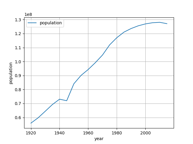
今回は日本の全国の総人口の推移を使って線形回帰をしてみましょう。
データは以下のサイトの全国の男女別人口のファイル(2015年に調査された、大正9年~平成27年のものを使用しました。)を使用します。 csv形式による主要時系列データ e-Stat - 政府統計の総合窓口
ダウンロードするとc02.csvの名前で保存されていると思うので、それをPythonを起動するディレクトリと同じ所に移動します。これで前準備完了です。
データの中身をプロットする
まずはデータの中身を確認してみます。
In [1]: import pandas as pd

In [3]: df = pd.read_csv('c02.csv', encoding="shift_jis") # utf-8では読み込めないので個別に指定する

In [4]: df.head() # まずは少しだけ中身を覗く
Out[4]:
   元号  和暦(年)   西暦(年)  年齢5歳階級      人口(総数)       人口(男)       人口(女)
0  大正    9.0  1920.0      総数  55963053.0  28044185.0  27918868.0
1  大正    9.0  1920.0    0〜4歳   7457715.0   3752627.0   3705088.0
2  大正    9.0  1920.0    5〜9歳   6856920.0   3467156.0   3389764.0
3  大正    9.0  1920.0  10〜14歳   6101567.0   3089225.0   3012342.0
4  大正    9.0  1920.0  15〜19歳   5419057.0   2749022.0   2670035.0
データを見ると、階級ごとの年齢が出ていますが今回欲しいのは総数だけです。
総数の部分だけ抜き出してみます。
In [5]: population = df[df['年齢5歳階級']=='総数']

In [6]: population.head()
Out[6]:
    元号  和暦(年)   西暦(年) 年齢5歳階級      人口(総数)       人口(男)       人口(女)
0   大正    9.0  1920.0     総数  55963053.0  28044185.0  27918868.0
19  大正   14.0  1925.0     総数  59736822.0  30013109.0  29723713.0
38  昭和    5.0  1930.0     総数  64450005.0  32390155.0  32059850.0
57  昭和   10.0  1935.0     総数  69254148.0  34734133.0  34520015.0
76  昭和   15.0  1940.0     総数  73075071.0  36540561.0  36534510.0
西暦と、人口だけ抜き出して、プロットします。
In [7]: population = population[['西暦(年)','人口(総数)']]

In [8]: population.columns = ['year', 'population']

In [9]: population.head()
Out[9]:
      year  population
0   1920.0  55963053.0
19  1925.0  59736822.0
38  1930.0  64450005.0
57  1935.0  69254148.0
76  1940.0  73075071.0

In [10]: import matplotlib.pyplot as plt

In [11]: population = population.set_index('year') # インデックスを西暦年にする。

In [12]: population.plot()
Out[12]: <matplotlib.axes._subplots.AxesSubplot at 0x10f8e2f98>

In [13]: plt.ylabel('population')
Out[13]: Text(0,0.5,'population')

In [14]: plt.xlabel('year')
Out[14]: Text(0.5,0,'year')

In [15]: plt.grid()

In [17]: plt.show()
表示されるグラフな以下のようになります。
OLSで線形回帰をする
それでは最小二乗法(OLS)を用いた線形回帰をします。 statsmodels のOLSというメソッドを使います。
In [18]: import statsmodels.api as sm

In [21]: model = sm.OLS(population.population, sm.add_constant(population.index)).fit() # 回帰分析

In [22]: model.params # population = year * x1 + const ということになる
Out[22]:
const   -1.589481e+09
x1       8.580823e+05
dtype: float64

In [30]: population.plot() # ここからグラフのプロットをしていく
Out[30]: <matplotlib.axes._subplots.AxesSubplot at 0x10b434828>

In [32]: plt.plot([1920,2015], model.predict(sm.add_constant([1920,2015])), label='prediction') # 先ほど求めたモデルの予測値をプロットする。(1920~2015)の間で。
Out[32]: [<matplotlib.lines.Line2D at 0x11483d240>]

In [33]: plt.xlabel('year')
Out[33]: Text(0.5,0,'year')

In [34]: plt.ylabel('population')
Out[34]: Text(0,0.5,'population')

In [35]: plt.grid()

In [36]: plt.title('population with prediction')
Out[36]: Text(0.5,1,'population with prediction')

In [37]: plt.legend()
Out[37]: <matplotlib.legend.Legend at 0x10dd35da0>

In [39]: plt.show()
グラフは以下の通りです。
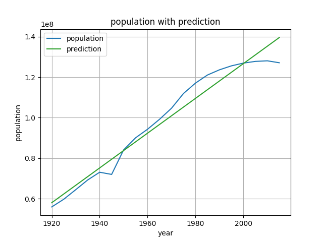
sm.add_constantを使わないと直線近似の際、うまく切片を求めてくれないからです。
求めたパラメーターを元に、手動で予測値を求めてもみましょう。
単純な線形結合なので、先ほど求めたパラメーター名x1とconstを使うと、
で求めることができるはずです。
In [32]: plt.plot([1920,2015], model.predict(sm.add_constant([1920,2015])), label='prediction')
Out[32]: [<matplotlib.lines.Line2D at 0x11483d240>]

In [33]: plt.xlabel('year')
Out[33]: Text(0.5,0,'year')

In [34]: plt.ylabel('population')
Out[34]: Text(0,0.5,'population')

In [35]: plt.grid()

In [36]: plt.title('population with prediction')
Out[36]: Text(0.5,1,'population with prediction')

In [37]: plt.legend()
Out[37]: <matplotlib.legend.Legend at 0x10dd35da0>

In [39]: plt.show()
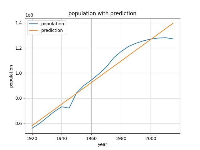 あまり面白みのない直線ですが、とりあえず予測することができました。
サマリーを表示させて概要を確かめてみます。
In [51]: print(model.summary())
                            OLS Regression Results
==============================================================================
Dep. Variable:             population   R-squared:                       0.959
Model:                            OLS   Adj. R-squared:                  0.957
Method:                 Least Squares   F-statistic:                     424.1
Date:                Fri, 14 Sep 2018   Prob (F-statistic):           5.81e-14
Time:                        12:00:00   Log-Likelihood:                -337.26
No. Observations:                  20   AIC:                             678.5
Df Residuals:                      18   BIC:                             680.5
Df Model:                           1
Covariance Type:            nonrobust
==============================================================================
                 coef    std err          t      P>|t|      [0.025      0.975]
------------------------------------------------------------------------------
const      -1.589e+09    8.2e+07    -19.386      0.000   -1.76e+09   -1.42e+09
x1          8.581e+05   4.17e+04     20.593      0.000    7.71e+05    9.46e+05
==============================================================================
Omnibus:                        1.640   Durbin-Watson:                   0.342
Prob(Omnibus):                  0.440   Jarque-Bera (JB):                0.964
Skew:                          -0.536   Prob(JB):                        0.617
Kurtosis:                       2.923   Cond. No.                     1.34e+05
==============================================================================

Warnings:
[1] Standard Errors assume that the covariance matrix of the errors is correctly specified.
[2] The condition number is large, 1.34e+05. This might indicate that there are
strong multicollinearity or other numerical problems.
多項式でフィッティング
次は多項式でフィッティングさせてみます。
例として2次式でフィッティングさせてみましょう。
多項式の場合はstatsmodels.formula.apiをインポートします。
ここでは予測させたいモデルを設定することができ、
formula = '求めたい値 ~ 予測したいモデル'
という形で指定することになります。
Rに近いスタイルの指定の仕方です。
例えば、今回の場合変数’year’を使った二次式のモデルを予測させたいので、二次の部分を関数functionに入れて
def function(year):
  return year * year

formula = 'population ~ year * function(year)'
という風に指定します。あくまでそれぞれの項の係数を求めていくので二次以上の項を入れたい場合は関数に入れる必要があります。
In [53]: import statsmodels.formula.api as smf # statsmodeld.formula.apiをインポート

In [58]: population = population.reset_index() # インデックスを列データに戻す

In [59]: population.head()
Out[59]:
     year  population    prediction
0  1920.0  55963053.0  5.803712e+07
1  1925.0  59736822.0  6.232753e+07
2  1930.0  64450005.0  6.661795e+07
3  1935.0  69254148.0  7.090836e+07
4  1940.0  73075071.0  7.519877e+07

In [62]: def function(year): # 二次の項は関数で設定
    ...:     return year * year
    ...:

In [64]: model = smf.ols(formula = 'population ~ year + function(year)', data=population).fit()

In [65]: model.params # 求められたパラメーターをみる
Out[65]:
Intercept        -2.113389e+10
year              2.072960e+07
function(year)   -5.049940e+03
dtype: float64
では、予測結果をグラフにプロットしていきます。
In [68]: plt.plot(population['year'],population['population'],label='population')
Out[68]: [<matplotlib.lines.Line2D at 0x1147caf28>]

In [71]: plt.plot(population.year, model.predict(population.year),label='prediction')
Out[71]: [<matplotlib.lines.Line2D at 0x1147d54e0>]

In [72]: plt.xlabel('year')
Out[72]: Text(0.5,0,'year')

In [73]: plt.ylabel('population')
Out[73]: Text(0,0.5,'population')

In [75]: plt.grid()

In [76]: plt.legend()
Out[76]: <matplotlib.legend.Legend at 0x1147cf630>

In [78]: plt.show()
このプロットの結果は以下のようになります。
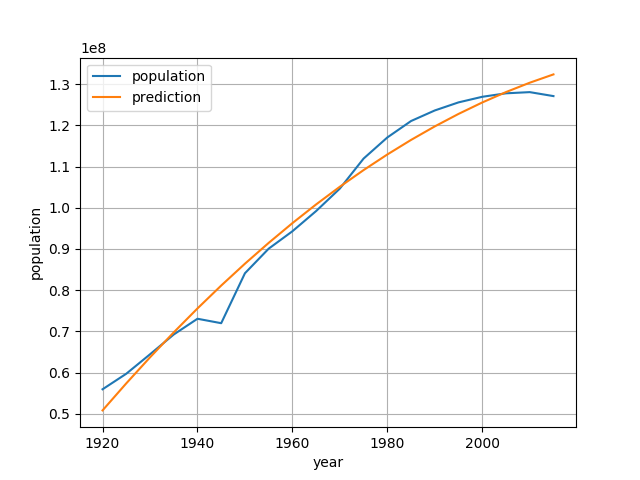
少しだけカーブが加わったので若干実際のものに近づいている感じがします。
まとめ
今回はPandasとstatsmodelsを使った線形回帰の手法についてまとめました。 予測自体は非常にシンプルなコードで書けてしまい、むしろグラフのプロットのコードの量が多い結果となりました。
かなり手軽に実装できるので線形回帰をさせたいという時はstatsmodelsを使って見ることをオススメします。他にも色々な統計的な機能を備えているので気になる方は是非調べてみてください。